Two Papers

Robustness and Security in ML Systems, Spring 2021

Jonathan Soma

January 19, 2021

Handwritten Digit Recognition with a Back-Propagation Network

Y. Le Cun, B. Boser, J. S. Denker, D. Henderson, R. E. Howard, W. Hubbard, and L. D. Jackel

a.k.a. Le Cun 1990

Yann LeCun

Yann LeCun on Wikipedia

Chief AI Scientist (and several other titles) at Facebook, “founding father of convolutional nets.”
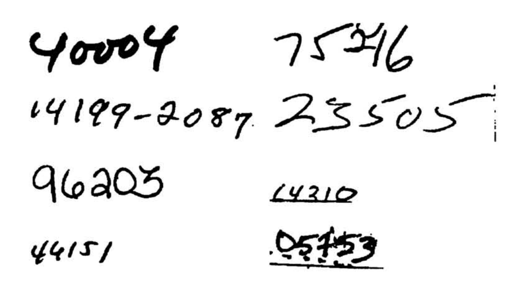
Yann Le Cun vs. Yann LeCun

All kinds of badly programmed computers thought that “Le” was my middle name. Even the science citation index knew me as “Y. L. Cun”, which is one of the reasons I now spell my name “LeCun”.

From Yann’s Fun Stuff page

Also: Falsehoods Programmers Believe About Names

The Problem

How to turn handwritten ZIP codes from envelopes into numbers
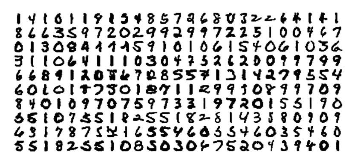
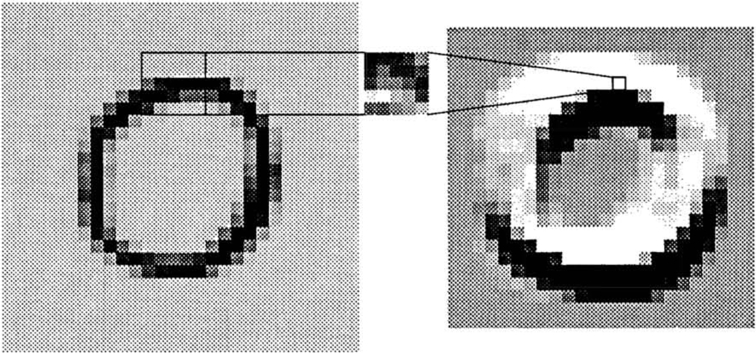
Examples of original zipcodes from the testing set

NOT The Problem

  • Location ZIP code on the envelope
  • Digitization
  • Segmentation

ONLY concerned with converting a single digit’s image into a number

Examples of normalized digits from the testing set

Network Input

Digitized zero

Input: 16x16 grid of greyscale values, from -1 to 1

Normalized from ~40x60px original, preserving aspect ratio. Network needs consistent size!

Network Output

To a human: Potential classes of 0, 1, 29

To the computer: Ten nodes, activated from -1 to +1. Higher value means higher probability of it being that digit. More or less one-hot encoding.

For example

Given the output

[0 0 0.5 1 0 -0.3 -0.5 0 0.75 0]

The network’s prediction is nine because 0.75 is the highest number. Next most probable is a three with a score of 0.5.

Four Hidden Layers

  • Input: 16x16 greyscale input
  • H1: Feature layer
  • H2: Averaging layer
  • H3: Feature layer
  • H4: Averaging layer
  • Output: 10x1 encoding

Not fully-connected. “A fully connected network with enough discriminative power for the task would have far too many parameters to be able to generalize correctly.”

Convolution

A convolution is used to “see” patterns around a pixel like horizontal, vertical or diagonal edges.

A 3x3 kernel being applied to an image

It’s just linear algebra: a kernel is applied to create a new version of a pixel dependent on the pixels around it. The kernel (or convolutional matrix) is just a matrix that is multiplied against each pixel and its surroundings.

Application of the convolution

Edges of the image are padded with -1 to allow kernel to be applied to outermost pixels. The result is called a feature map.
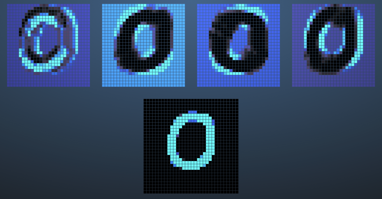
Kernel being applied to create the first layer

A single kernel map

The -1 +1 range of each feature map highlights a specific type of feature at a specific location.
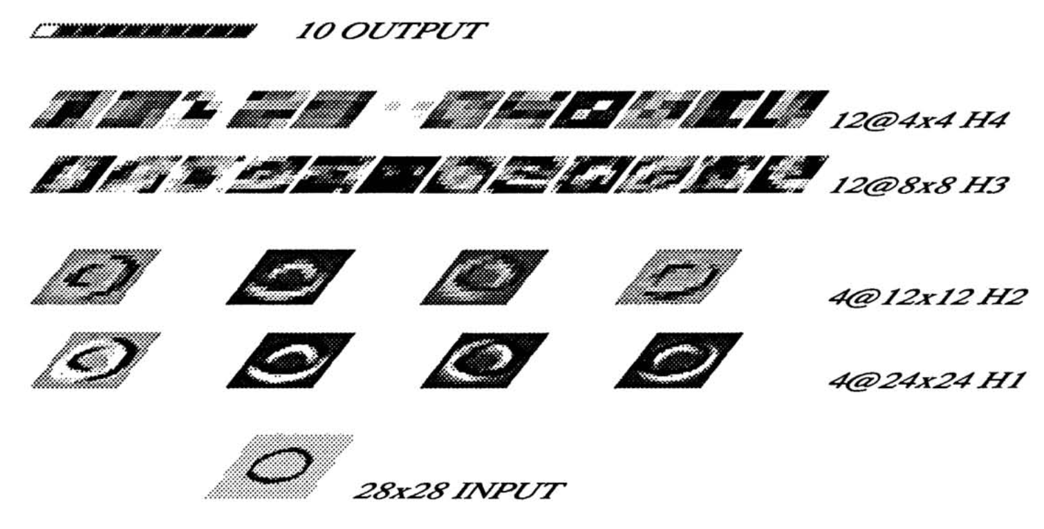
Upper edge highlighted by a convolution

Layer: H1

Four different 5x5 kernels are applied, creating four different 576-node feature maps that each highlight a different type of feature.
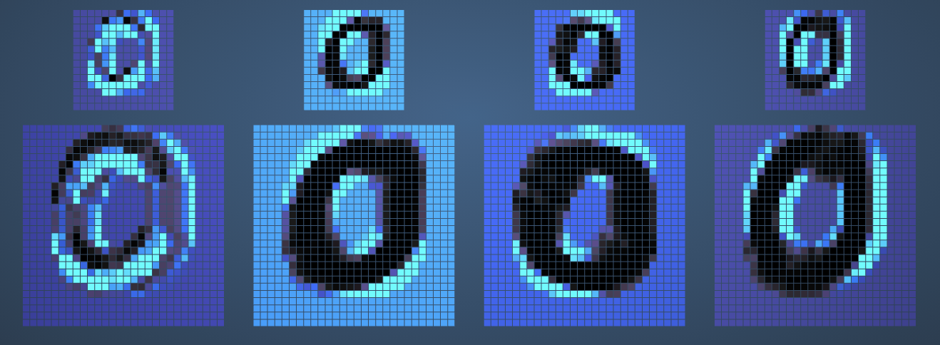
Four kernels applied, each extracting a different feature

Layer: H2

We don’t need all that detail, though! Layer H2 averages the 24x24 feature maps down to 12x12, converting local sets of 4 nodes in H1 to a single node in H2.

Reducing layer H2

Layer: H3

H3 is another feature layer, operating just like H1 but with 12 8x8 feature maps. Each kernel is again 5x5.
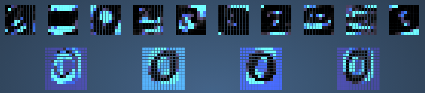
Feature layer H3

H2-H3 connections

Note that not all H3 kernels are applied to all H2 layers. Selection is “guided by prior knowledge of shape recognition.” This simplifies the network.

Connections between H2 and H3 layers

Layer: H4

H4 is similar to H2, in that it averages the previous layer. This reduces H3’s 8x8 size to 4x4.

Reducing layer H4

Output

10 nodes, fully connected to H4. Each activates between -1 and +1 with a higher score meaning a more likely prediction for that digit.

The complete network as illustrated by the paper

Overall

  • 4,635 nodes, 98,442 connections, 2,578 independent parameters
  • Did not depend on elaborate feature extraction, only rough spatial and geometric information.

Training and testing

  • Trained on 7,291 handwritten + 2,549 printed digits with 30 epochs.
  • Test set error rate was 3.4%.
  • Errors were half due to faulty segmentation, and some human beings couldn’t even read!

Performance

Example of atypical data

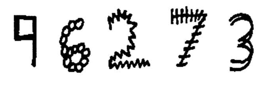
Robust model that generalizes very well when presented with unusual representations of digits.

Throughput is mainly limited by the normalization step! Reaches 10-12 classifications per second.

Sources

// reveal.js plugins